2011-09-29

Objects in Javascript and Python

I've been doing some Javascript recently (well, Coffeescript actually, but this applies equally to either, so I'll stick to Javascript for the examples) and found its approach to objects rather interesting. I think it might be instructive to compare Javascript's objects to Python's, the dynamic programming language I'm most familiar with.

First of all, take this Javascript code, which creates a factory-function called "Counter" which returns objects with "increment" and "decrement" methods:

function Counter() {
    this.value = 0
}
Counter.prototype.increment = function() {
    this.value += 1;
}
Counter.prototype.decrement = function() {
    this.value -= 1;
}
c1 = new Counter()
c2 = new Counter()
c2.increment()

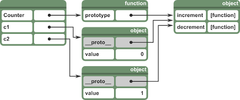
When we execute it, we end with a set of objects much like this:

In our outermost scope (the identity of which I'll gloss over for now) we have three names (or keys) defined. "Counter" is a function object, while "c1" and "c2" are both generic objects. "Counter", like all functions, has an object attached to it under the key "prototype", and it's in this prototype object that we've inserted the functions increment and decrement.

Each time we invoke "new Counter()" a new object is created with its special "__proto__" key mapped to Counter.prototype, and then the Counter function is executed with "this" bound to the new object. The Counter function adds to that object, mapping "value" to the number 0. (I must say, I still don't entirely understand why "new" works like this - I can't see any value in being able to invoke the same function both with and without "new".)

Finally we invoke "c2.increment()". First Javascript looks on the c2 object for the key "increment", but there is no such key. Next, it follows the "__proto__" key and tries again with the prototype object. There it finds the increment function. The function is executed with "this" bound to the "c2" object. When it does "this.value += 1" it first looks up "value" in the same way, finding it directly on the object itself, then after adding 1 to the value it stores it back on the object. (Note that storing something doesn't involve "__proto__" traversal. It always goes straight into the object that you put it into. It's only look-ups that involve "__proto__" traversal.)

Now, let's see the same thing in Python:

class Counter(object):
    def __init__(self):
        self.value = 0
    def increment(self):
        self.value += 1
    def decrement(self):
        self.value -= 1
c1 = Counter()
c2 = Counter()
c2.increment()

At a first glance, things look pretty similar. The "__class__" attributes on the objects are much like the special "__proto__" attributes in Javascript. The "__init__" method is quite similar to the "Counter" function in Javascript. The differences are subtle.

When Python executes the class statement, the three functions "__init__", "increment" and "decrement" are defined and attached to the newly created class object.

When "Counter()" is invoked a bunch of stuff goes on behind the scenes, but importantly a new object instance is created with "__class__" pointing to the class and then the "__init__" function is invoked with the object instance as its first argument.

When "c2.increment()" is executed, first "increment" is looked up on c2. This fails, so next Python follows "__class__" and checks for "increment" on the class. However, something special happens when it finds it there. When an attribute lookup for an object finds a function on its class object, it instead returns a "bound method", which is effectively a function that takes one fewer argument then passes through to the "increment" function itself, inserting a reference to the object as the first argument. So even though the statement "c2.increment()" provides no arguments, when "increment" is actually executed, it receives c2 as its first argument.

There are, I think, two interesting differences here. One is what happens when we want to represent inheritance, which my example doesn't really cover. In Javascript, if attribute lookup fails on the prototype then the prototype's prototype is searched, and so on. In Python, if the attribute lookup fails on the class, then instead of looking at its "__class__" attribute, the base classes are searched. (And since Python allows multiple inheritance, the corner cases are a bit tangled.)

But what I think is most interesting are the different approaches to how methods know their receiving object and the unintuitive consequences of these mechanisms. In Javascript, when a function is retrieved from an object and invoked on the same expression, it triggers the binding of "this" to the object in the function. But if you take a reference to the function and invoke it separately then "this" remains "undefined". For example:

c1.increment();

is not equivalent to this:

var f = c1.increment;
f();

The former will increment c1. The latter will do nothing because increment executes with this undefined.

In Python, on the other hand, the equivalent will work as you might expect, because "c1.increment" in fact refers to a bound method. However, from this we can see that in Python "Counter.increment" is not the same entity as "c1.increment". "Counter.increment" is a function that takes one argument. "c1.increment" is a bound method that takes no arguments. In contrast, in Javascript, "Counter.prototype.increment" refers to the exact same object as "c1.increment". So Python does the magic during object attribute lookup, while Javascript does the magic when invoking an attribute as a function.

I think this is all correct, but do let me know if I've made a mistake. I'm finding Javascript a lot more pleasant than I expected, except for its cheerful silent propagation of "undefined" at every opportunity, and Coffeescript definitely rounds off some of the rough corners. In fact, I'd say I even slightly prefer Coffeescript's class notation to Python's.

I'm curious to know if there are any particular benefits of prototype-based objects. I can't see any clear advantages over class-based objects, and I particularly don't understand the benefit of being able to use any function to create an object. Is it just nice because it results in a smaller language? (Does it result in a smaller language?)
2011-07-18

As if by magic, some maths appeared

I've not really done any programming lately, so this week there's no Minecraft. Instead there's some maths. Hurrah! Hey, where are you—

I was reading Richard Wiseman's Friday puzzle. It's very short and not at all hard, so you might want to go and solve it and come back. Go on, I'll wait.

Okay, you're back? I'll try not to state the answer outright, but it will probably become pretty obvious very quickly. Right, so this got me thinking about sums of series. The case in the question is sufficiently small that you don't even need to work out the formula for the sum of sequence in question, but I was thinking about it nonetheless.

Now, I knew the formula for the sum of an arithmetic sequence, and I knew that you could easily enough prove it by induction, but this is a very unsatisfying form of proof. It doesn't feel like something you could have figured out on your own. Imagine just picking random equations one at a time and testing them until you find one that you can prove correct with induction! I thought about it a little and came up with what I thought was a pretty compelling geometric proof, at least for the simple case where you start at 1 and increment by 1. (I have no idea if a proper mathematician would call this a proof. I am certainly not a proper mathematician.)

Is it obvious? On the left in the green we have a square with area 1, a rectangle with area 2, a rectangle with area 3, etc. The area of the whole shape must be the sum of those areas. By dividing up the space differently, we can easily see how to produce the closed form.

Great, I thought. Now lets do the same for the sum of squares. It must be just as obvious in 3D. Right?

Hmmm. Well, it gives the right answer, and it's satisfying to figure it out by hand, but it lacks the obviousness of the diagram for the arithmetic sequence sum. Perhaps there's a simpler way to do it?

As an aside, I think I'm getting the hang of Inkscape, although there are still some areas I find I much prefer Visio. Inkscape has some pretty painful and inflexible handling of arrowheads, for example. They're always black, regardless of the line colour, and then there's a special menu action just to make them change to match the line colour. The selection of arrowheads available is limited and weird, and most of them aren't resizable. I'm not sure if that's because SVG forces arrowheads to behave in strange and unintuitive ways, or that's just the way that Inkscape chooses to work.

Maybe next week there will be more programming. We shall see.

2011-07-12

Minecraft mapping - Rotation and flipping

Last time, I discussed ambient occlusion for adding depth to the map. Today I'm going to explain how the fragment shader rotates and flips oriented blocks like minecart tracks.

As you may have noticed, there's only one block ID for regular minecart tracks. The 4-bit data value encodes the orientation of the track, from 10 possibilities - 2 orientations of straight track, 4 orientations of corner track, and 4 orientations of sloped track.

A minecraft texture pack includes only two textures for normal minecart tracks: one curved and one straight. We need to use these to make up all the other orientations. We could either do that in advance - building up a bigger texture atlas with all the orientations we need, or we can do it in the shader. By doing it in the shader we avoid the need for a much expanded texture atlas and some fiddly work to assemble textures, at the cost of extra work in the shader.

To let the shader know what orientation to use, we encode it in the blue channel of our map data texture. We use 2 bits to encode a rotation (0°, 90°, 180° 270°) and 1 bit to encode a possible flip. (I don't think we actually use the flip at the moment, but it might be useful for doors.)

The shader code isn't actually terribly exciting. I should however point out that this version treats the map texture as having normalized float values, rather than integers. For most of the earlier posts I had been updating the code to use integer textures to simplify things a bit, but I haven't gotten around to doing that with this code. That's why we multiply the sample values by 255.0 – as normalized floats they've already been rescaled from 0 to 255 to the range 0.0 to 1.0.

    float flipx = (tiles_sample.b * 255.0) >= 8.0 ? -1.0 : 1.0;
    float rotation = mod(
        tiles_sample.b * 255.0, 8.0) *
        0.5 * 3.141592653589793;
    mat2 transform = mat2(
        flipx * cos(rotation),  flipx * sin(rotation),
        -sin(rotation),         cos(rotation));

We form a rotation matrix with the rotation value of 0, 0.5π, π or 1.5π. The sines and cosines just work out as -1, 0 or +1. There's probably a cheaper way to calculate them.

This will rotate around the origin. Before we transform our texture coordinate we rescale it to the range -1..1, then adjust it back afterwards.

Some mention should be given to how we obtain the rotation values in the first place. There's no trick – there's just a great big table mapping block id and data values to texture coordinates and orientations. The same table is used to pick coloured wool values.

And here's the end result. I think I've talked about most of the things I had originally set out to cover. Next week I might touch on light levels, but there's not a lot to say there. If I find the time I'd like to do some work on cave rendering, but I'm not sure I'll both find the time to work on it and write a blog post, so next week's post may be quite short.

2011-07-05

Minecraft mapping - Ambient occlusion 2

Last time I described in principle how the ambient occlusion shader works, but didn't really go into the details. Today I'll go into a bit more detail.

Something that I think may not have been clear last time is that we're calculating ambient occlusion independently from lighting based on the "blocklight" and "skylight" values. For ambient occlusion we're considering only the arrangement of solid blocks in the immediate neighbourhood, not any genuine sources of light. As a separate step we later multiply together the ambient occlusion value and the light-level based on blocklight and skylight. Again, this is a simplification, and it does result in extra shadows in dark areas, but it generally looks fine.

As we saw previously, to determine the the level of shadow added by occlusion, we determine how much "sky" is visible from the rendered surface, where the sky is actually a horizontal square not very far above the surface. This screenshot shows the view from the ground looking up. The white blocks represent the sky square, and the stone slabs are neighbouring taller cells.

The yellow outline shows the unoccluded area of sky. The following diagram breaks that down into the areas shadowed by each of the eight neihbouring columns:

Area A is the occlusion from a neighbouring corner block, while areas B and C are occlusions from neighbouring side blocks. You'll observe that 1. the corner blocks always occlude rectangular regions of sky; 2. the side blocks occlude trapezoidal areas and 3. the corner block occlusions can overlap with the neighbouring side blocks.

Now, I have to admit that I made a bit of a mistake when I first worked this out, and didn't realise that the side blocks were occluding trapezoids, so I worked it as if they were rectangles instead, like this diagram:

The problem with making this as a simplification is that it will result in significant discontinuities around corners. Encountering these, but not understanding why, I experimented with tweaking values and if you look in the shader code you'll see a comment, "TODO: Figure out why the 2* multiplier is needed in the next line!" I haven't actually figured out why that works yet, but I plan to work through the maths again with trapezoids, if it's not too complicated, and see how it compares. However, for now I'm going to discuss the slightly broken version with the rectangles.

Here's another pair of diagrams of those occlusion rectangles:

On the left we have a similar case with some extra occluding columns. Things to note here are that the yellow corner column provides no extra occlusion because it is shorter than both of the neighbouring side columns. The dotted line shows the division of the sky square into quadrants, each of which we'll handle separately.

On the right diagram, you can see the same arrangement, but different rectangles are highlighted. The orange "+" rectangle is the area of unoccluded sky in the quadrant ignoring the corner column. This can be easily calculated based on the proximity of the neighbouring cells on the sides, and the heights of the columns in those cells. The teal "−" rectangle is the extra occlusion provided by the corner column, which we subtract from the unoccluded area to find the total unoccluded area in the quadrant. We calculate the teal area similarly, using the proximity of the neighbouring side cells, and the height of the corner column, but we make sure to clamp its dimensions to be positive – if either dimension would be negative it means the corner block is not going to provide any occlusion and can be ignored.

I've left this a bit late, so I don't have formatted code snippets or a nice runnable example, but you can go look at the complete fragment shader in github. The obscurely named "lightcalc" calculates the dimension of one side of the orange rectangle based on the height and proximity of the neighbouring cell, with 1 being the maximum unoccluded size. "cornerlight" calculates the unoccluded area in the quadrant, again with 1 being entirely unoccluded.

This shader is pretty slow. It results in a noticeable frame-rate drop for me. I haven't yet investigated whether the cost is in the quantity of calculations or from sampling all eight neighbouring cells for their height, but I suspect it's the latter. If that's the case, we could preprocess the image and store information about each cell's neighbours in a compressed form, reducing the number of samples needed. Maybe an expert could suggest the most fruitful avenues to optimization.

Here's what it looks like without any textures:

Any thoughts? It occurs to me that I could very well have overlooked a much easier or a less horrifically simplified way to do this. I'll need to look into how feasible it is to properly calculate the trapezoidal areas, and also figure out why the bodge of doubling the teal area results in continous results (at least, continuous between cells of equal height; we don't want continuity across height changes – the whole point of this is to highlight height differences). Feel free to ask questions if it's not clear. I may yet do one more post on this topic if people would like further clarification.

2011-06-28

Minecraft mapping - Ambient occlusion

Today I'm going to talk about the approach to ambient occlusion used in the Minecraft mapper.

First of all, we assume that light falls uniformly from the sky, like on an overcast day. The amount of light illuminating a particular patch of ground is thus proportional to the amount of the sky that can be seen unobstructed from that point. The following diagrams show the general idea in 2D from the side:

The red point on top of a plateau has an unobstructed view of the sky, so it is maximally illuminated. The green point is only slightly occluded by the peak on the left. The blue point is substantially occluded on both sides, so it will be quite dark.

That's the general idea. The amount of illumination for every point will be proportional to the solid angle of the sky visible from that point. However, that's quite a lot of work to do. We're going to cheat a lot by making a number of simplifications:

  • We're going to ignore overhead obstructions and only consider the occlusion caused by neighbouring cells.
  • We're going to assume that the sky is in fact a horizontal plane 3m above the point we're rendering.
  • We're further going to consider only a 2m×2m square of that plane, and assume that the visible 2D area of that square is a reasonable approximation of the solid angle of sky visible from the point.

The following diagram gives an idea of what we're talking about, again looking at things side-on:

The reason these simplifications help is that we can now calculate the occlusion just from a height-field describing the heights of the cells that we're rendering. For each pixel, we consider the height of the cell it's in and the height of the neighbouring cells. For each neighbouring cell, we consider how much higher it is than the central cell, and how far the edge of that cell is horizontally from the point being rendered. Based on all that, we can calculate how much of the 2m square patch of sky is visible.

In this diagram the red point is a pixel for which we want to calculate the ambient occlusion. The pixel is very close to the tall cell to the north, which will occlude a fair bit of the sky. The medium sized block to the east is a bit further away and not as tall, so it won't occlude as much, and might not occlude any at all. The only other taller block, to the south-west, is sufficiently far away and small that it's not going to occlude any of the patch of sky we're considering.

Next time I might go over the maths, or I might set this aside for now and talk about how we flip and rotate tiles for rendering minecart tracks. Let me know if you have a preference.

2011-06-21

Minecraft mapping - Using NumPy to flatten the map

Previously, we put together some code to render a 2D array of tiles. But rendering a horizontal 2D slice of the 3D Minecraft world is not particularly helpful. Today we will use numpy to flatten the 3D terrain into a 2D map.

Essentially, we just want to cast a bunch of vertical rays towards the ground and find the spots where they meet the ground:

Note in particular that we want to allow the starting point to be in solid matter, and when it is, we don't want it to end until it first exits the solid matter and then hits the ground. This makes it easier to see relatively shallow caverns in amongst great depths of rock. In addition, we're going to allow specifying a height-field for the ray-starts. I think this will be useful later for mapping multi-level underground structures - I'm imagining either letting the user paint across the map with a "deeper" and a "shallower" brush, or calculating a starting height-field based on one or more seed points.

The blue ray doesn't hit any floor in the specified range. That's a cell that we'll either leave transparent or render some sort of "wall" texture into.

These two diagrams show different height-fields selected to catch different floors. Whereas the first image had some abrupt changes when the height-field of ray sources passed through floors, here we've avoided that by slightly changing the height-field.

That's the theory behind using a height-field here. In practice I haven't done much with the height-fields yet other than test that they work by making diagonal slices through the world.

This is the method on Volume that takes two height-fields, a low-limit one that specifies how far we let the rays go, and a high-limit one that specifies what height we shoot the rays from. It outputs another height-field of which cells contain the floors we want to render, and a Boolean mask array that distinguishes where we found floors from where we found none. Note that the input height-fields can be simple scalars - if so, they're expanded out to make height fields.

    def get_floor_heights_and_mask(
            self,
            low_limit,
            high_limit,
            include_transparent=True):
        low_limit_3d = numpy.atleast_3d(low_limit)
        high_limit_3d = numpy.atleast_3d(high_limit)

We use numpy.atleast_3d to extend the height-field (or height scalar) into a 3D array. This adds extra dimensions of size 1, and allows numpy to "broadcast" when we use it in an operation with another 3D array with large size.

        max_height = self.blocks.shape[2]
        shape = self.blocks.shape
        trimmed_shape = (shape[0], shape[1], shape[2]-1)
        cell_depth = numpy.indices(trimmed_shape)[2]

This creates cell_depth as a 3D array of the same size as the volume except one cell shallower, and with each cell having a value equal to its depth. (Actually, "depth" is a bit misleading. It increases in the upward direction. "Altitude" may have been more appropriate.)

        cell_is_selected = numpy.logical_and(
                cell_depth >= low_limit_3d,
                cell_depth < high_limit_3d)

This creates a Boolean array of the same dimensions that is true for the cells that fall within the range between our height-fields.

        selectable_substance = (
                self.blocks[:,:,:-1]
                if include_transparent
                else numpy.logical_not(
                    tileid_is_transparent[self.blocks[:,:,:-1]]
                )
            )

This takes all the blocks in the volume, minus the very top layer. We're going to use it in a Boolean expression shortly, so all that matters is if it's 0 or not. This method is used twice, once to search for non-transparent blocks, and again to search for partially transparent blocks. So when "include_transparent" is true, we just use the values of the blocks themselves, which will be non-zero for all cells apart from air. When "include_transparent" is false, we use a look-up table to decide whether each block is of a transparent or non-transparent type.

        potential_floors = numpy.logical_and(
                selectable_substance, cell_is_selected
            )
This creates "potential_floors" as another 3D Boolean array, where true cells indicate that there's a block we might want to render that's within the range of the ray. But this will still select multiple cells in any given vertical column...
        potential_footspace = (
                self.blocks[:,:,1:]
                if include_transparent
                else numpy.logical_not(
                    tileid_is_transparent[self.blocks[:,:,1:]]
                )
            )
We define "potential_footspace" almost identically to "potential_floors", but it's shifted one cell upward.
        good_floors = numpy.logical_and(
                potential_floors!=0,
                potential_footspace==0)

Now we construct "good_floors" out of "potential_floors" and "potential_footspace", selecting all those cells in range where a solid cell has a transparent cell immediately above it. If we think back to the rays being cast, this corresponds to every point where the ray passes from air into a floor. We may still be selecting multiple cells in any given vertical column.

        floor_heights = (
                (max_height - 2) -
                numpy.argmax(good_floors[:,:,::-1], axis=2)
            )

Here numpy.argmax does the magic. We're applying it to a Boolean array. In the case of ties, it always selects the cell with the lowest index. So if there are a mix of true and false values, it will pick the lowest index cell containing true, otherwise it will pick index 0. Since we actually want the highest index cell, we use a negative stride slice ("::-1") to vertically flip the array before the calculation.

        mask = get_cells_using_heightmap(
                good_floors, floor_heights)
        return (
                numpy.clip(floor_heights, low_limit, high_limit),
                mask
            )

Finally we calculate the mask by checking whether the cells we finally selected were previously identified as suitable floors, and we clamp our floor heights to fall within our specified range. I've forgotten now why we need to clamp the floor heights. Perhaps that's now redundant.

I'm sorry this is a bit brief. I think I'm going to continue this once a week instead of twice, with posts on Tuesdays, because I don't think I can quite keep up the same pace, and I'm spending a lot of the time I would have used to experiment with new code just putting together the posts and their diagrams.

Please feel free to ask questions if there's anything you're curious about, or make suggestions about better ways to do things. I think there are quite a lot of bits that could be a lot more elegant, especially where the code has grown very organically and still has odd the odd vestigial appendix that has become quite redundant.

2011-06-17

Minecraft mapping - Applying Minecraft textures

Last time we loaded a Minecraft file and rendered a big grid of numbers indicating the block ID of cells in the map. Those block IDs don't directly tell us which item in the texture atlas to use. Instead, we create a great big mapping table that says for each block ID which texture from the texture atlas to use. That's still not going to be perfect - for wool blocks we also need to consider the data value to pick the colour. For minecart tracks the data value will tell us the orientation of the tracks, but then we only have two textures - one straight and one corner! In the future we'll see how to write a pixel shader that flips and rotates them appropriately. Other blocks like signs and torches and doors don't have any appropriate texture for rendering a top-down view, so we'll need to create them. Most evil of all is redstone wire - for one thing, the orientation of the wire isn't encoded in the saved game at all – we need to calculate it by looking at surrounding tiles. In addition, Minecraft renders redstone wire using a small number of textures and some rather complicated operations to clip and colour them. I haven't yet tackled that problem, and I might just avoid it.
Today all we do is use the mapping table to look up the position in the texture atlas (which I'm calling the "texture code") for blocks from the same slice of the map as last time. I'm not going to discuss that in detail because it's not terribly exciting. Pull down the code from github, and copy your terrain.png file into the same directory before you run texture_demo.py. (I don't think I can legally include terrain.png in the repo unless I draw it all myself.) You'll see something like this:
Here you can see pink squares in areas of empty space, tree trunks, leaves in dark grey, grass in light grey, dirt in brown and stone in medium grey. The reason that the leaves and grass are grey is because the texture in terrain.png is greyscale and Minecraft colours it at run-time based on the biome. We might do that eventually, but it's probably easier just to use a custom terrain.png with green leaves and grass.
One thing that I would like to discuss is some of the stuff we're doing in numpy that's not really important just now, but will be much more important when we render more than just a flat horizontal slice of the world.
def get_cells_using_heightmap(source, heightmap):
    '''
    Given a 3D array, and a 2D heightmap, select cells from the
    3D array using indices from the 2D heightmap.
    '''
    idx = [numpy.arange(dimension) for dimension in source.shape]
    idx = list(numpy.ix_(*idx))
    idx[2] = numpy.expand_dims(heightmap, 2)
    return numpy.squeeze(source[idx])
We use this function to flatten the 3D array of blocks into a 2D array. Note that I will be referring to the dimensions of the 3D array as X, Z and Y, in that order, to match how Minecraft lays them out. The funcion is pretty hideous, but I couldn't find anywhere describing an easier way to do this in numpy. I think I found it here. Looking at it again I really don't like that it reuses the name idx to mean rather different things. Basically, it works like this:
  • Supposing the input array "source" is 512×512×128, we first construct three arrays, [0, 1, 2 ... 510, 511], [0, 1, 2 ... 510, 511] and [0, 1, 2 ... 126, 127].
  • We then feed them into numpy.ix_, which converts them into 3D arrays. The first has dimensions 512×1×1, the second 1×512×1 and the last 1×1×128, and each has the sequence of values that we previously fed in.
  • We throw away the third one and replace it with our height-field. If our height-field has less than two dimensions, we bump it up to two dimensions. (This lets us pass in a single value if we want a uniform height-field.)
  • The horrifying magic occurs when we use this bizarre collection of three arrays as the indices into source. First of all, numpy applies its broadcasting rules to expand all of index arrays to have matching dimension. The result of this is that all three of our indexing arrays end up with dimensions 512×512×1.
  • The dimensions of the indexing arrays determine the dimensions of the result of the indexing operation. Each element of the output array is determined by looking up the source array with the coordinates from the indexing arrays at the corresponding position. The X and Z indexing arrays basically just pass through the X and Z coordinates unmodified. The Y indexing array is our height field.
  • Finally, we use numpy.squeeze to discard the last dimension.
Now that I've spent the time to think about it and explain it, I think it could be made clearer. I think the use of ix_ followed by broadcasting is quite hard to follow. I think we could avoid the extra dimension and the squeeze too. I don't think there's any getting around the fancy indexing.
That's quite enough for today. I'm now undecided what I'll discuss next week. I'm really not sure who's reading and what sort of interests they have. Are you beginners or experts? Do you want tutorials and stuff that you can easily try at home, or would you prefer a faster paced tour of the fancy bits? Is it important to build things up a step at a time or would you prefer I skip over things to get to the good stuff? How painful is this numpy stuff? I could spend some time drawing up diagrams to better explain it, but that would probably mean it will be quite a while before we get to the interesting shader stuff. Let me know what you think in the comments.
Next time: using numpy to flatten the map.


2011-06-14

Minecraft mapping - Reading Minecraft files

(Part of a series on rendering top-down Minecraft maps.)
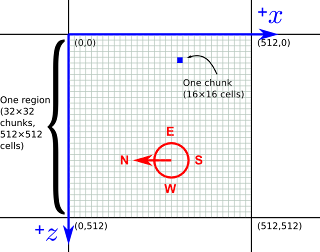
For storage, the current version of Minecraft breaks the world up into 512×512 cell regions and breaks regions up into 16×16 cell chunks. (These are the X×Z dimensions, regions and chunks are both a full 128 cells tall in the Y dimension.) Previous versions stored each chunk as a separate NBT file, but recent versions bundle up a whole region of chunks into a single MCR file. We can use this NBT parser for Python, but (as far as I can tell) it doesn't know anything about MCR files.
MCR files are really just containers for compressed NBT files. The format is described here: Beta Level Format. We can use that information to seek to the compressed chunk data, decompress it, then feed the decompressed data to the NBT parser.
def read_nbt_from_mcr_file(mcrfile, x, z):
    """
    Read NBT chunk (x,z) from the mcrfile.
    0 <= x < 32
    0 <= z < 32
    """
    #read metadata block
    block = 4*(x+z*32)
    mcrfile.seek(block)
    offset, length = unpack(">IB", "\0"+mcrfile.read(4))
    if offset:
        mcrfile.seek(offset*4096)
        bytecount, compression_type = unpack(
                ">IB", mcrfile.read(5))
        data = mcrfile.read(bytecount-1)
        decompressed = decompress(data)
        nbtfile = NBTFile(buffer=StringIO(decompressed))
        return nbtfile
    else:
        return None
The parsed NBT file gives us access to various pieces of data. This is described here: Chunk file format. We're most interested in "Blocks", the array of block IDs for the blocks in the chunk. Later on we'll also need "Data", because this distinguishes subtle details of certain blocks, such as the colour of wool blocks and the orientation of minecart track blocks. "SkyLight" and "BlockLight" will let us apply lighting to blocks based on illumination from the sky (skylight) and from torches, lava, glowstone and so on (blocklight).
To better manipulate this data, we're going to put it in a numpy array. We use a 3D "structured array" with fields for each of the four pieces of data we've identified. The class VolumeFactory provides various methods that create volumes:
class VolumeFactory(object):
    def empty_volume(self, dimensions):
        data = numpy.zeros(
            dimensions,
            dtype = [
                ('blocks', 'u1'),
                ('data', 'u1'),
                ('skylight', 'u1'),
                ('blocklight', 'u1')])
        return Volume(data)
Empty volume just creates a volume containing 0 for every field. It uses numpy.zeros to create a structured array of the appropriate dimensions.
    def load_chunk(self, nbtfile, volume=None):
        if volume is not None:
            if volume.dimensions != (16,16,128):
                raise TypeError(
                    "load_chunk requires a volume "+
                    "that is 16x16x128")
        if nbtfile is None:
            if volume is None:
                return self.empty_volume((16,16,128))
            volume.blocks[:,:,:]=0
            volume.skylight[:,:,:]=0
            volume.blocklight[:,:,:]=0
            volume.data[:,:,:]=0
            return volume
        if volume is None:
            volume = self.empty_volume((16,16,128))
        level = nbtfile['Level']
        blocks = arrange_8bit(level['Blocks'].value)
        skylight = arrange_4bit(level['SkyLight'].value)
        blocklight = arrange_4bit(level['BlockLight'].value)
        data = arrange_4bit(level['Data'].value)
        volume.blocks[:, :, :] =  blocks
        volume.skylight[:, :, :] = skylight
        volume.blocklight[:, :, :] = blocklight
        volume.data[:, :, :] = data
        return volume
Apart from the handling for non-existent chunks, load_chunk takes an already-loaded NBT file, and uses arrange_4bit and arrange_8bit to assemble that data into the numpy arrays. (Numpy doesn't allow elements crammed together on boundaries smaller than 1 byte, so we pad the 4-bit values out to 8-bits.)
    def load_region(self, fname):
        f = open(fname, "rb")
        region = self.empty_volume((512,512,128))
        chunk = self.empty_volume((16,16,128))
        for z in xrange(32):
            for x in xrange(32):
                chunkdata = read_nbt_from_mcr_file(f, x, z)
                self.load_chunk(chunkdata, volume=chunk)
                region[16*x:16*(x+1), 16*z:16*(z+1), :] = chunk
        return region
Finally, load_region calls load_chunk repeatedly for the 32×32 chunks in a region. It uses numpy's array slicing to paste them together into one big array. Many regions won't be fully-explored, and so many of the chunks will be missing. Those are just filled in with zeroes.
The main program is largely unchanged from last week's zooming and panning one. All that is changed is how we fill the "minecraft_map" texture:
    volume_factory = VolumeFactory()
    region_volume = volume_factory.load_region(
            'world/region/r.0.0.mcr')
    map_rgb_array = numpy.zeros((512,512,3), dtype="u8")
    map_rgb_array[:,:,0] = region_volume.blocks[:,:,70]
    minecraft_map = make_surface(map_rgb_array)
Here I load a minecraft region from a region file I have on my computer called "world/region/r.0.0.mcr". You can find your own region files on your Minecraft saves folder. (On Linux this is in "~/.minecraft/saves", I'm not sure where it ends up on other systems. Perhaps %APPDATA% on Windows.) For now, since we're not yet doing anything smart to flatten the Minecraft map, we just take a slice at y=70. This is just a little bit above sea-level, so it contains a mix of air and land. You can see the results in the annotated screenshot below:
As before, the full code is up on github. The new files are "minecraft_mapping.py" and "nbt_demo.py", the latter of which can be run. You'll need to edit it though, because the path to the Minecraft region file is hard-coded and you'll want to point it towards one of your own map files.
On Friday, we'll look at applying Minecraft's own textures to the map, and next week we'll get on to flattening the 3D map data into something (moderately) useful for a map.


2011-06-10

Minecraft mapping - Zooming and panning

Last time we did some tiled rendering. However, it was pretty awkward to look at the results because we needed to edit the code and re-run it if we wanted to move around. Today we add zooming and panning controls.
Before we start looking at the details, I should point out that all the code is now available on github. That includes the previous two examples "opengl1.py" and "opengl2.py", as well as today's, "zoompan.py". If you look in there you can see everything I've written for this project, but be aware that most of it is very haphazard. I'm brushing off and tidying up the corresponding parts as I write each article. Feel free to ask questions about any of the code in there, but please don't beat me up too much for my coding style!
Most of the changes this time are to the main loop:
def main(): 
    video_flags = OPENGL|DOUBLEBUF
    pygame.init()
    screen_dimensions = 800, 600
    surface = pygame.display.set_mode(
        screen_dimensions, video_flags)
    resources = make_resources()
    frames = 0
    done = 0
    zoom = 1.0
    position = [256, 8192 - 256]
    dragging = False
    draglast = 0,0

    while not done:
        while 1:
            event = pygame.event.poll()
            if event.type == NOEVENT:
                break
            if event.type == KEYDOWN:
                pass
            if event.type == QUIT:
                done = 1
            if event.type == MOUSEMOTION:
                if dragging:
                    mx,my = event.pos
                    lx,ly = draglast
                    dx = (mx - lx)/zoom
                    dy = (my - ly)/zoom
                    position[0] -= dx
                    position[1] += dy
                    draglast = mx, my
            if event.type == MOUSEBUTTONDOWN:
                if event.button == 1:
                    draglast = event.pos
                    dragging = True
                if event.button == 4:
                    zoom *= 2.0
                    if zoom > 16:
                        zoom = 16.0
                if event.button == 5:
                    zoom /= 2.0
                    if zoom < 1.0/32.0:
                        zoom = 1.0/32.0
                    x,y = position
                    x = math.floor(x * zoom + 0.5) / zoom
                    y = math.floor(y * zoom + 0.5) / zoom
                    position = [x,y]
            if event.type == MOUSEBUTTONUP:
                if event.button == 1:
                    dragging = False
        render(resources, position, zoom, screen_dimensions)
        frames += 1

if __name__ == '__main__':
    main()
As you'll probably have noticed, all the code for rendering from a different position and zoom factor was already there. All we need to do is add handling for the mouse events that appropriately updates the camera position and zoom factor. Mouse buttons 4 and 5 are triggered by the scroll wheel. When it rolls up we double the zoom factor, and when it rolls down we halve it.
Mouse button 1 is the left (or primary) button. When it is pressed down we enter dragging mode and when it is released we leave dragging mode. Whenever the mouse moves in dragging mode, we track how far it moved and update the camera position, taking into account the zoom factor. Note that for mouse events the y coordinate increases down the screen, while our camera y increases up the screen.
One last thing to note is that when zooming out, we apply rounding to the camera position. This is so that every pixel matches up perfectly with a texel. When I didn't have this, sometimes if you zoomed in, panned around and then zoomed out you'd see odd pixels at the boundaries between tiles.
The other minor changes this time are to use mipmapping. This involves some changes to how we set up our texture atlas:
    glTexParameteri(
        GL_TEXTURE_2D,
        GL_TEXTURE_MIN_FILTER,
        GL_NEAREST_MIPMAP_NEAREST)
    glTexParameteri(
        GL_TEXTURE_2D,
        GL_GENERATE_MIPMAP,
        GL_TRUE);
As I understand it, GL_GENERATE_MIPMAP is deprecated, but the alternative – the glGenerateMipmap function – isn't in PyOpenGL's OpenGL.GL module. I didn't really look into it much. I assume that it's either from a newer version of OpenGL than PyOpenGL supports, or it's in some obscure submodule.
I'm using GL_NEAREST_MIPMAP_NEAREST as the minification function. This means that we don't do any interpolation - we just pick the closest mipmap level and in that mipmap level pick the closest texel. This is fine because our zoom levels are powers of 2 and we keep the texels and pixels lined up. It also avoids some ways for things to go wrong.
The shader also needs a change:
fragcolor = textureGrad(
    texture_atlas, atlas_point,
    vec2(1/512.0/zoom,0), vec2(0,1/512.0/zoom));
Instead of using the texture function, we use textureGrad. This lets us give the GPU a hand in choosing a mipmap level. Without it, mipmap levels are chosed by looking at how much the texture coordinates are changing between one screen pixel and the next. This works fine in the middle of our tiles, but fails at the edges, because our texture coordinates jump suddenly between one tile and another. You can see in the image on the right inappropriate mipmap levels on the borders of tiles. There should be no borders between tiles!
The extra parameters for textureGrad allow us to specify the rate of change of the texture coordinates per pixel both horizontally and vertically. We can calculate them based on the zoom level.
You can get the current version of the code from github. Next week, we'll start looking at reading Minecraft maps. We'll be using an NBT parser for Python with some extra work to read the region files used by recent versions of Minecraft. (Well, recent at the time of writing.)


2011-06-07

Minecraft mapping - Tiled rendering

This is the fourth in a series of articles about my attempts to write a Minecraft mapping program using Python. Last week, we made a simple texture and rendered it with OpenGL. For the amount of work involved, it wasn't terribly impressive! Today we're going to change the fragment shader to do the tiled rendering that we described before.
The fragment shader needs to calculate what colour each pixel should be. As input, it takes the texture coordinates that were output by the vertex shader. We have a single great big square with texture coordinate (0,0) in the bottom left and texture coordinate (1,1) in the top right. We want to texture this with a 512×512 grid of square textures drawn from our 16×16 grid of textures in our texture atlas.
The fragment shader needs to do two things with the texture coordinate. One is to look up our 512×512 texture that is our Minecraft map region - it can do that directly with no extra calculation. The other is to take that texture coordinate, consider it as a point in a grid of 512×512 cells, and figure out where it falls within its cell. We call this position theta. A theta of (0,0) corresponds to the bottom left of the cell, and (1,1) to the top right of the cell.
Given the sample taken from our map texture, we extract the red value to get a code between 0 and 255 that indicates a cell in our texture atlas. We call the position of that cell phi. The bottom-left cell in the texture atlas has phi=(0,0), the top-right cell has phi=(15, 15).
Finally, combining phi and theta identifies the position to sample from the texture atlas for the fragment we're rendering. Here's the new shader:
fragment_shader = '''\
#version 130

const float TILE_COUNT = 512.0;
const float INV_TILE_COUNT = 1.0 / TILE_COUNT;

uniform sampler2D texture_atlas;
uniform usampler2D map_texture;

in vec2 texcoord;
out vec4 fragcolor;

void main()
{
    vec2 theta;

    
    theta = (mod(texcoord, INV_TILE_COUNT) * TILE_COUNT);
    uvec4 map_sample = texture(map_texture, texcoord);
    uint uphi = map_sample.x % 16u;
    uint vphi = 15u - (map_sample.x / 16u);
    vec2 phi = vec2(uphi, vphi);
    vec2 atlas_point = phi / 16.0 + theta / 16.0;

    fragcolor = texture2D(texture_atlas, atlas_point);
}
'''
The complete source file is here:opengl2.py There are a few other changes. I've also tried enabled mip-mapping on the texture atlas, while limiting it to four levels, because beyond that the mip-maps would start blending together unrelated tiles. Unfortunately, I think I've still not quite got it working right, but that won't be immediately obvious. I might talk about it more in a later article, but it's going to need some work.
Here's the end result. (Click it to view it full size.) As you'll note, for now we've used the diagnostic texture for both the map texture and the texture atlas. On Friday we'll add some controls to zoom and pan so that we can actually see the whole thing and next week we'll start reading from Minecraft files.


2011-06-03

Minecraft mapping – Rendering with PyOpenGL

Last time we made ourselves a simple texture using Pygame. Today we're going to render it as-is on the screen using PyOpenGL. Simple, right?
This will probably be a little steep if you don't know any OpenGL. However, fear not. Read An intro to modern OpenGL by Joe Groff. It's great, and it's how I learned to write GLSL shaders. Well, I say learned to write them – I've pretty much only written the one that you're going to see in these articles. The tutorial's in C, but I've translated the early parts into Python: Python OpenGL tutorial Lastly, don't worry if the 3D maths is scary – we won't be needing it since we're sticking solidly to 2D. (That said, I am quite scared of the maths in the ambient occlusion bit. But we'll worry about that when we come to it.)
In addition to Python and Pygame, you're going to need PyOpenGL and NumPy. I installed them on Ubuntu using:
sudo apt-get install python-opengl
sudo apt-get install python-numpy
(This should all work fine on Windows and Mac, but you'll need to download and install all these things separately.)
#!/usr/bin/env python

# Copyright 2011, Annette Wilson
# Licensed under the MIT license:
# http://www.opensource.org/licenses/MIT
#
# Minecraft mapping - Rendering something with OpenGL
#
# With great thanks to Joe Groff:
# http://duriansoftware.com/joe/An-intro-to-modern-OpenGL.-Chapter-1:-The-Graphics-Pipeline.html

from OpenGL.GL import *
import pygame, pygame.image, pygame.key
from pygame.locals import *
from opengl_tools import *

vertex_shader='''\
#version 130

uniform vec2 screen_dimensions;
uniform vec2 cam_position;
uniform float zoom;
uniform float texture_dimension;
uniform float map_dimension;

in vec4 position;
out vec2 texcoord;

void main()
{
    gl_Position.xy =
        (
            (position.xy / 2.0 + 0.5)
            * texture_dimension
            - cam_position
        )
        * 2.0
        * zoom
        / screen_dimensions;
    gl_Position.zw = vec2(0.0, 1.0);
    texcoord = position.xy * 0.5 + 0.5;
}
'''
Our square sits between (-1,-1,0) and (1,1,0) in world space. Screen space has (-1,-1) as the bottom-left of the screen and (1,1) as the top-right. If the texture is texture_dimension pixels across, and cam_position is a set of pixel coordinates in texture, this will position the square so that the given pixel is in the centre of the screen. We also use the original world space coordinates as the texture coordinates, but we multiply by 0.5 and add 0.5 because we want the texture coordinates to range from 0 to 1. So the bottom-left of our texture will have texture coordinates (0,0) and the top-right will have (1,1).
fragment_shader = '''\
#version 130

uniform sampler2D texture_atlas;
uniform usampler2D map_texture;

in vec2 texcoord;
out vec4 fragcolor;

void main()
{
    fragcolor = texture2D(texture_atlas, texcoord);
}
'''
The fragment shader is even more trivial. We just look up the texture atlas texture. Next time we will develop this to do something more interesting.
class Resources(object):
    pass

def make_resources():
    minecraft_map = pygame.Surface((512,512))
    atlas = pygame.image.load('numbered_texture_atlas.png')
    vertex_buffer_data = float_array(
        -1.0, -1.0, 0.0, 1.0,
         1.0, -1.0, 0.0, 1.0,
        -1.0,  1.0, 0.0, 1.0,
         1.0,  1.0, 0.0, 1.0)
    element_buffer_data = short_array(
        0,1,2,3)
    resources = Resources()
    resources.vertex_buffer = make_buffer(
        GL_ARRAY_BUFFER,
        vertex_buffer_data,
        vertex_buffer_data.nbytes)
    resources.element_buffer = make_buffer(
        GL_ELEMENT_ARRAY_BUFFER,
        element_buffer_data,
        element_buffer_data.nbytes)
    resources.map_texture = make_texture(
        image=minecraft_map, interpolate=False,
        alpha=True, integer=True)
    resources.texture_atlas = make_texture(
        image=atlas, interpolate=False, alpha=True)
    resources.program = assemble_shader_program(
        vertex_shader,
        fragment_shader,
        uniform_names=[
            'screen_dimensions',
            'cam_position',
            'zoom',
            'texture_dimension',
            'texture_atlas',
            'map_texture'],
        attribute_names=[
            'position'])
    return resources
This sets up all the resources we need:
  • map_texture is a placeholder for our map data. We'll make use of this next time.
  • texture_atlas is the texture atlas that we created last time.
  • vertex_buffer contains the four vertices of our square.
  • element_buffer is a list of indices into vertex_buffer_data, describing the order they should be connected up in a triangle strip.
  • program is our shader program, combining the vertex and fragment shaders.
This makes use of various helper functions we define in opengl_tools.py.
def render(resources, position, zoom, screen_dimensions):
    screen_w, screen_h = screen_dimensions
    glViewport(0,0,screen_w,screen_h)
    glClearColor(0.4, 0.4, 0.4, 1.0)
    glClear(GL_COLOR_BUFFER_BIT)

    glUseProgram(resources.program.program)
    uniforms = resources.program.uniforms
    glUniform2f(uniforms['screen_dimensions'], screen_w, screen_h)
    glUniform2f(uniforms['cam_position'], position[0], position[1])
    glUniform1f(uniforms['zoom'], zoom)
    glUniform1f(uniforms['texture_dimension'], 512.0) 

    glActiveTexture(GL_TEXTURE0)
    glBindTexture(GL_TEXTURE_2D, resources.map_texture)
    glUniform1i(resources.program.uniforms['map_texture'], 0)

    glActiveTexture(GL_TEXTURE1)
    glBindTexture(GL_TEXTURE_2D, resources.texture_atlas)
    glUniform1i(resources.program.uniforms['texture_atlas'], 1)

    glBindBuffer(GL_ARRAY_BUFFER, resources.vertex_buffer)
    glVertexAttribPointer(
        resources.program.attributes['position'],
        4, # size
        GL_FLOAT, # type
        GL_FALSE, # normalized?
        ctypes.sizeof(GLfloat)*4, # stride
        None # offset
        )
    position_attribute = resources.program.attributes['position']
    glEnableVertexAttribArray(position_attribute)
    glBindBuffer(GL_ELEMENT_ARRAY_BUFFER, resources.element_buffer)
    glDrawElements(
        GL_TRIANGLE_STRIP,
        4,
        GL_UNSIGNED_SHORT,
        None)
    glDisableVertexAttribArray(position_attribute)
    pygame.display.flip()
Given the simplicity of the shaders, rendering is a somewhat gruesome affair. We need to provide a value for each of the uniforms that we defined in the shaders, bind textures to slots, connect up and enable a vertex array on each attribute and finally draw our triangle strip.
def main(): 
    video_flags = OPENGL|DOUBLEBUF
    pygame.init()
    screen_dimensions = 800, 600
    surface = pygame.display.set_mode(
        screen_dimensions, video_flags)
    resources = make_resources()
    frames = 0
    done = 0
    zoom = 1.0
    position = [256.0, 256.0]
    dragging = False
    draglast = 0,0

    while not done:
        while 1:
            event = pygame.event.poll()
            if event.type == NOEVENT:
                break
            if event.type == KEYDOWN:
                pass
            if event.type == QUIT:
                done = 1
        render(resources, position, zoom, screen_dimensions)
        frames += 1

if __name__ == '__main__':
    main()
And this is the output. Not thrilling, I'll admit, but I wanted to get as much of the tedious stuff out of the way to avoid confusing things too much when we do more with the shaders. You can download the two files from github. Next time: tiled map rendering.